Topic Overview

Measures of Central Tendency

---

1. Definition of Central Tendency

Core Definition

• A measure of central tendency is a single value that represents the center of a dataset
• It gives an idea about the typical or average value

---

Key Concepts

• Summarization of data
  • Converts large data into a single representative value
• Representative value
  • Reflects the overall pattern of the dataset

---

Easy Example

• Data: 2, 4, 6, 8, 10
• Central value → around 6
  → This represents the dataset

---

2. Types of Central Tendency ⭐

---

Mean (Arithmetic Mean)

---

Definition

• The mean is the average of all observations
• It is calculated by dividing the sum of values by number of observations

---

Formula ⭐

xˉ=∑xn\bar{x} = \frac{\sum x}{n}xˉ=n∑x​

---

For Grouped Data ⭐

xˉ=∑fx∑f\bar{x} = \frac{\sum f x}{\sum f}xˉ=∑f∑fx​

---

Easy Explanation

• Add all values → divide by total number
• For grouped data → multiply frequency with value

---

Example

• Data: 2, 4, 6, 8
• Mean = (2+4+6+8) / 4 = 5

---

Important Exam Points ⭐

• Most commonly used measure
• Affected by extreme values (outliers)

---

Median

---

Definition

• Median is the middle value after arranging data in ascending or descending order

---

Method of Calculation ⭐

Odd Number of Observations

• Median = value at position
  (n + 1) / 2

---

Even Number of Observations

• Median = average of two middle values
  n/2 and (n/2 + 1)

---

Worked Example ⭐

Odd Case

• Data: 1, 3, 5, 7, 9
• Median position = (5+1)/2 = 3rd value
• Median = 5

---

Even Case

• Data: 2, 4, 6, 8
• Middle values = 4 and 6
• Median = (4+6)/2 = 5

---

Easy Understanding

• Median divides data into two equal halves
• Not affected by extreme values

---

Important Exam Points ⭐

• Median = middle value
• Requires arrangement of data
• Preferred when data has outliers

---

Short Note (Revision)

• Mean → average
• Median → middle value
• Mean affected by outliers
• Median not affected

 

 

Mode

---

Definition

• Mode is the most frequently occurring value in a dataset
• It represents the value that appears maximum number of times

---

Easy Explanation

• Data: 2, 4, 4, 6, 8
• Mode = 4 (appears most frequently)

---

Characteristics ⭐

• May not be unique
  • Dataset can have:
    • One mode → Unimodal
    • Two modes → Bimodal
    • More → Multimodal
• Useful in categorical data
  • Best for qualitative data
  • Example:
    • Most common blood group
    • Most common disease
• Not affected by extreme values
  • Outliers do not influence mode

---

Important Exam Points ⭐

• Mode = most frequent value
• Useful for categorical data
• May have multiple modes

---

Short Note (Revision)

• Most frequent value
• Can be multiple
• Useful in qualitative data

 Characteristics of a Good Average ⭐

---

Essential Features

• Simple to understand
  • Should be easy for anyone to interpret
• Easy to calculate
  • Calculation should not be complicated
• Based on all observations
  • Should consider entire dataset
• Not affected by extreme values
  • Should be stable even if outliers are present
• Capable of further analysis
  • Should be useful for:
    • Statistical calculations
    • Comparisons
    • Research analysis

---

Easy Understanding

• A good average should be:
  • Simple + reliable + representative

---

Important Exam Point ⭐

• Ideal average = simple, stable, representative, and usable for analysis

---

Short Note (Revision)

• Simple
• Easy to calculate
• Uses all data
• Not affected by extremes
• Useful for analysis

 

 

Mean ⭐

---

Properties

• Uses all data values
  • Every observation contributes to the mean
• Affected by extreme values (outliers)
  • Very high or low values can distort the mean

---

Advantages

• Mathematical usefulness
  • Can be used for:
    • Further calculations (SD, variance, regression)
• Stability
  • Less fluctuation in repeated samples

---

Disadvantages

• Influenced by outliers
  • Not suitable for skewed data

---

Quick Example

• Data: 2, 4, 6, 8, 100
• Mean = 24 → not representative due to outlier

---

Median ⭐

---

Properties

• Not affected by extreme values
  • Outliers do not change median
• Divides data into two equal halves
  • 50% values below, 50% above

---

Advantages

• Suitable for skewed data
  • Best when extreme values are present

---

Disadvantages

• Does not use all observations
  • Only depends on middle value

---

Quick Example

• Data: 2, 4, 6, 8, 100
• Median = 6 → more representative

---

Mode

---

Properties

• Most frequent value
  • Highest occurrence in dataset

---

Advantages

• Useful for nominal/categorical data
  • Example:
    • Most common blood group
    • Most common disease

---

Disadvantages

• May be multiple or no mode
  • Data may be:
    • Bimodal
    • Multimodal
    • No mode

---

Quick Example

• Data: 2, 4, 4, 6, 8
• Mode = 4

---

High-Yield Comparison (Exam Trick) ⭐

Mean

• Uses all data
• Affected by outliers
• Best for symmetrical data

Median

• Middle value
• Not affected by outliers
• Best for skewed data

Mode

• Most frequent value
• Used for categorical data
• May not be unique

---

Short Note (Revision)

• Mean → average (affected by extremes)
• Median → middle (stable)
• Mode → most frequent

 

Feature	Mean	Median	Mode
Definition	Sum of all values ÷ number of observations	Middle value after arrangement	Most frequent value
Data Used	Uses all observations	Does not use all values fully	Based on frequency
Effect of Outliers	Affected	Not affected	Not affected
Best Use	Symmetrical data, further calculations	Skewed data	Categorical/qualitative data
Example	Average marks	Income distribution	Most common blood group

 

 

Skewness ⭐

---

Definition

• Skewness is the measure of asymmetry of a distribution
• It shows whether data is symmetrically distributed or shifted to one side

---

Easy Explanation

• If data is evenly spread → Symmetrical
• If tail extends to right/left → Skewed distribution

---

Types of Skewness ⭐

---

1. Symmetrical Distribution

• Data is evenly distributed on both sides
• Mean = Median = Mode

---

2. Positive Skew (Right Skew)

• Tail extends towards right side
• Few high extreme values present
• Relationship:
  • Mean > Median > Mode

---

3. Negative Skew (Left Skew)

• Tail extends towards left side
• Few low extreme values present
• Relationship:
  • Mean < Median < Mode

---

Diagrams (VERY IMPORTANT) ⭐

 

 

 

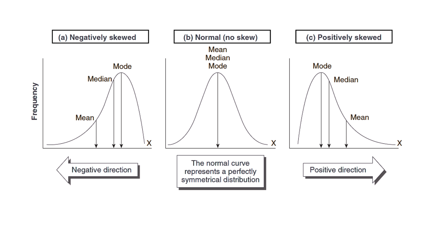
4

---

Interpretation ⭐

Direction of Skewness

• Right tail → Positive skew
• Left tail → Negative skew

---

Clinical / Epidemiological Examples

• Positive Skew
  • Income distribution (few very high incomes)
  • Hospital stay duration (few long stays)
• Negative Skew
  • Age at death in developed countries (most live longer)
• Symmetrical
  • Normal distribution (e.g., height in population)

---

Important Exam Points ⭐

• Skewness = asymmetry of distribution
• Formulas to remember:
  • Positive skew → Mean > Median > Mode
  • Negative skew → Mean < Median < Mode

---

Short Note (Revision)

• Symmetrical → Mean = Median = Mode
• Positive skew → Right tail
• Negative skew → Left tail

 

 

Measures of Dispersion

---

Definition of Dispersion

Core Definition

• Dispersion is the measure of spread or variability of data
• It shows how far the values are scattered from the central value

---

Easy Explanation

• Same mean, different spread:

  Data 1: 5, 5, 5, 5 → No dispersion
  Data 2: 1, 5, 9, 5 → High dispersion

---

Importance ⭐

• Shows reliability
  • Less dispersion → data is more reliable
• Indicates consistency
  • Small spread → consistent data
  • Large spread → variable data

---

Types of Dispersion ⭐

---

1. Range

---

Definition

• Range is the difference between highest and lowest value

---

Formula ⭐

Range=Max−Min\text{Range} = \text{Max} - \text{Min}Range=Max−Min

---

Easy Example

• Data: 2, 4, 6, 8
• Range = 8 – 2 = 6

---

Advantages

• Simple and easy to calculate
• Quick idea of spread

---

Limitations

• Uses only two values (max & min)
• Not reliable
• Affected by outliers

---

2. Quartile Deviation (Semi-IQR)

---

Definition

• Based on quartiles (Q1 and Q3)
• Measures spread of middle 50% data

---

Formula ⭐

QD=Q3−Q12QD = \frac{Q_3 - Q_1}{2}QD=2Q3​−Q1​​

---

Easy Explanation

• Q1 → 25th percentile
• Q3 → 75th percentile
• Focuses on central data, ignores extremes

---

Advantages

• Not affected by extreme values
• Better than range

---

Limitations

• Does not use all data
• Limited mathematical use

---

3. Mean Deviation

---

Definition

• Mean deviation is the average of absolute deviations from mean or median

---

Easy Explanation

• Calculate how far each value is from mean
• Take average of those distances

---

Example (Concept)

• Data: 2, 4, 6
• Mean = 4
• Deviations: 2, 0, 2
• Mean deviation = (2+0+2)/3 = 1.33

---

Advantages

• Uses all observations
• Better than range

---

Limitations

• Absolute values → difficult for further calculations
• Less commonly used

---

Important Exam Points ⭐

• Range → simplest
• QD → middle spread
• Mean deviation → average distance

---

Short Note (Revision)

• Dispersion = spread of data
• Range → max – min
• QD → (Q3 – Q1)/2
• Mean deviation → average deviation

 

Standard Deviation (SD) ⭐ MOST IMPORTANT

---

Definition

• Standard deviation (SD) is a measure of variability of data around the mean
• It tells how much the values deviate (spread) from the average

---

Easy Explanation

• Small spread → values close to mean → low SD
• Large spread → values far from mean → high SD

---

Formula ⭐

For Individual Data

SD=∑(x−xˉ)2nSD = \sqrt{\frac{\sum (x - \bar{x})^2}{n}}SD=n∑(x−xˉ)2​​

---

For Grouped Data

SD=∑f(x−xˉ)2∑fSD = \sqrt{\frac{\sum f (x - \bar{x})^2}{\sum f}}SD=∑f∑f(x−xˉ)2​​

---

Easy Steps (Exam Trick)

1. Find mean (x̄)
2. Calculate (x − x̄)
3. Square → (x − x̄)²
4. Take average
5. Take square root

---

Interpretation ⭐

• Small SD
  • Data is closely clustered around mean
  • More consistent & reliable
• Large SD
  • Data is widely spread
  • Less consistency

---

Example

• Data 1: 5, 5, 5, 5 → SD = 0 (no variation)
• Data 2: 1, 5, 9, 5 → SD is high

---

Important Exam Points ⭐

• Most important measure of dispersion
• Uses all data values
• Essential for:
  • Normal distribution
  • Z-score
  • Statistical tests

---

Short Note (Revision)

• SD = spread around mean
• Small SD → consistent
• Large SD → variable

---

Variance

---

Definition

• Variance is the square of standard deviation
• It measures spread in squared units

---

Formula ⭐

Variance=SD2\text{Variance} = SD^2Variance=SD2

---

Easy Explanation

• Variance = average of squared deviations from mean
• SD = √Variance

---

Important Exam Points ⭐

• Variance = SD²
• Units are squared
• SD is preferred for interpretation

---

Short Note (Revision)

• Variance = square of SD
• SD more useful clinically

 

 

Properties of Standard Deviation ⭐

---

Key Properties

• Always positive
  • SD is never negative
  • Because deviations are squared before calculation
  • Minimum value = 0 (when all observations are same)

---

• Based on all observations
  • Every data value contributes to SD
  • Makes it a reliable measure of dispersion

---

• Affected by extreme values (outliers)
  • Very high or low values can increase SD significantly
  • Hence, SD is sensitive to skewed data

---

• Algebraically tractable
  • Can be used in mathematical/statistical calculations
  • Important for:
    • Variance
    • Z-score
    • Normal distribution
    • Regression & correlation

---

Easy Understanding

• SD = powerful + precise + mathematically useful
• But → sensitive to outliers

---

Important Exam Point ⭐

• SD is:
  • Always positive
  • Uses all data
  • Affected by outliers
  • Mathematically useful

---

Short Note (Revision)

• Always positive
• Uses all observations
• Affected by extremes
• Useful in calculations

 

 

Coefficient of Variation (CV) ⭐

---

Definition

• Coefficient of Variation (CV) is a relative measure of variability
• It expresses standard deviation as a percentage of mean
• Helps compare variability between different datasets

---

Formula ⭐

CV=SDxˉ×100CV = \frac{SD}{\bar{x}} \times 100CV=xˉSD​×100

---

Easy Explanation

• CV tells how large the variation is compared to the mean
• Lower CV → more consistency
• Higher CV → more variability

---

Uses ⭐

• Compare consistency between datasets
• Used when:
  • Means are different
  • Units are different

---

Example (Comparison) ⭐

Dataset A

• Mean = 100
• SD = 10

CV = (10 / 100) × 100 = 10%

---

Dataset B

• Mean = 50
• SD = 10

CV = (10 / 50) × 100 = 20%

---

Interpretation ⭐

• Dataset A → CV = 10% → More consistent
• Dataset B → CV = 20% → Less consistent (more variation)

---

Exam Trick ⭐

• Lower CV → Better consistency
• Higher CV → More variability

---

Important Exam Points ⭐

• CV = relative measure
• Used for comparison
• Expressed in percentage

---

Short Note (Revision)

• CV = (SD/Mean) × 100
• Lower CV → more stable
• Used to compare datasets

 

 

Normal Distribution & SD ⭐

---

Definition

• A normal distribution is a symmetrical, bell-shaped distribution
• Data is distributed evenly around the mean

---

Properties ⭐

• Mean = Median = Mode
  • All central tendencies coincide at the center
• Symmetrical distribution
  • Left side = Right side
• Total area = 100%
  • Entire curve represents 100% of data

---

Easy Explanation

• Most values lie near the mean
• Few values lie at extremes (tails)

---

Standard Deviation Distribution ⭐

• 68% of data → within ±1 SD
• 95% of data → within ±2 SD
• 99.7% of data → within ±3 SD

👉 This is called the Empirical Rule (68–95–99.7 rule)

---

Diagram (Bell-shaped Curve with SD Markings) ⭐

 

 

 

4

---

Interpretation ⭐

• Narrow curve → Small SD → Less variability
• Wide curve → Large SD → More variability
• Majority of values cluster around the mean

---

Clinical / Epidemiological Relevance

• Biological variables:
  • Height
  • Weight
  • Blood pressure
• Used in:
  • Reference ranges
  • Z-score calculations
  • Statistical tests

---

Important Exam Points ⭐

• Bell-shaped curve
• Mean = Median = Mode
• 68–95–99.7 rule (VERY FREQUENT MCQ)

---

Short Note (Revision)

• Normal distribution → symmetrical
• Mean = Median = Mode
• 68% → ±1 SD
• 95% → ±2 SD
• 99.7% → ±3 SD

 

Uses of Dispersion

---

Core Uses ⭐

• Measure reliability of data
  • Less dispersion → more reliable data
  • More dispersion → less reliable

---

• Compare datasets
  • Helps compare variability between two or more groups
  • Example: Using SD or CV to compare consistency

---

• Understand variability
  • Shows how much data values differ from the average
  • Helps identify spread and distribution pattern

---

Easy Example

• Dataset A → SD = 5 (less spread)
• Dataset B → SD = 20 (more spread)
  → Dataset A is more consistent

---

Public Health Applications ⭐

• Epidemiological studies
  • Assess variation in:
    • Disease occurrence
    • Risk factors

---

• Research interpretation
  • Helps interpret:
    • Study results
    • Clinical trial outcomes

---

Clinical Example

• Blood pressure readings:
  • Low SD → consistent readings
  • High SD → fluctuating readings

---

Important Exam Point ⭐

• Dispersion helps in:
  • Reliability
  • Comparison
  • Understanding variability

---

Short Note (Revision)

• Measures spread
• Helps compare datasets
• Indicates consistency
• Useful in epidemiology & research